A tool to visualize kernel header inclusion graphs.
These files are fairly large. I use gwenview on an Athlon64/3700 to display them with no problems.
There is a lot of information encoded in these graphs. This is a quick tutorial of what all the shapes, colors, and numbers mean. Most snapshots are taken from <linux/list.h> above.
Every graph is generated from a particular top level node. This node is shaped like a house and colored bright orange.
Like every other node, the root has 2 numbers in it, separated by a dash. The first number is the unique tsize, the second is the total tsize (these concepts are defined in the README.) In this case, <linux/list.h> includes, directly or indirectly, 51 unique header files. The other number is also important, but is rather less intuitive... best to just ignore it for the moment.
Note that the root node has no outgoing edges to the files it directly includes. These edges are snipped from the graph for layout purposes. The children of root are tagged with little orange asterisks so they are easy to find in the graph.
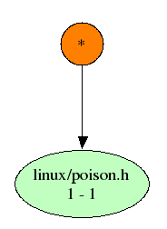
In this case, the included file is a nice, boring file which does not include any other files, so the unique tsize is 1 and it has no outgoing edges. In general, any file which does not significantly add to the size or complexity of the graph is colored green, like this one.
Some files add a lot of complexity to the graph by virtue of being very popular (lots of other files include them.) These files are colored yellow (or red, as we will see later).
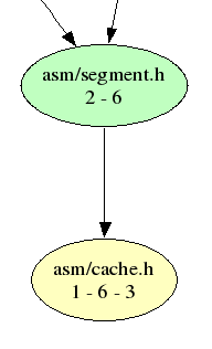
In this case, <asm/cache.h> is included from a total of 3 places. All but one of these edges has been removed for layout purposes. An additional number has been added after the tsizes to remind us of the total number of parents.
Snipped child nodes are apparent by their color, and by the fact that they have three numbers. However, it is important that we be able to recognize the snipped parents as well. This is done by making the parent nodes into boxes and listing the label of each missing child, one per row.
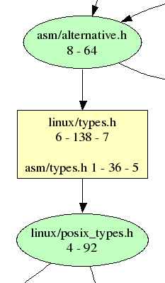
Looking at the node for <linux/types.h>, it is apparent that it includes, directly or indirectly, a total of 6 header files. It is a fairly popular file itself, having been included from 7 other places. Finally, it has two children, one from the visible edge and one in the list of snipped children. There is no indication on the graph about who the other 6 parent files are.
In this simple case, the unique tsize of <linux/types.h> (6) is just the sum of <linux/posix_types.h> (4), <asm/types.h> (1), and itself (1). In more complicated graphs, the children of a node may have partially overlapping inclusion trees, and the unique tsize of the node will be less than the sum of its children.
Nodes with a sufficiently large unique tsize are considered to be part of the "backbone" of the inclusion graph. These nodes are colored blue.
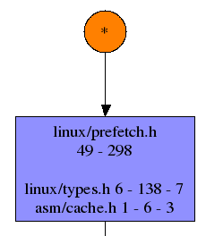
Looking at the graph, this node was included directly from the root node, but nowhere else. It directly includes a total of three other files, and indirectly includes a total of 49 unique header files.
This example is taken from <linux/sched.h> above.
Some nodes are included from all over the place, and they in turn include a large number of unique header files. These nodes are colored red, since they contribute significantly to the total complexity of the graph.
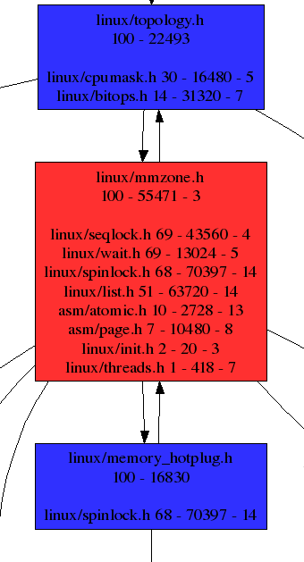
In this example, <linux/mmzone.h> is included from three different places, and includes 100 separate header files. Two of these links are cyclic, a case which the graph analyser detects and handles.
Note that the parent count for <linux/mmzone.h> is 3, but there are only two incoming edges rendered. This is because <linux/memory_hotplug.h> includes <linux/mmzone.h> twice.